A quick introduction to Probabilistic Graphical models

Introduction

Many complex systems, such as social networks, biological neurons, genomes, depend on many variables that in turn depend on each other in very complex ways. These dependencies are often only known to domain experts. To model these systems accurately, we need to encode the experts' beliefs about the dependency between individual variables, such as neuronal connectivity in the brain, or the connectivity of social networks.

For example, suppose you are trying to model the likelihood of an accident on a given day. And suppose that after looking at some data, you realize that the number of accidents spikes whenever:

1. The day happens to be a holiday.
2. The driver is under some type of influence.
3. The weather affects driving visibility.

Since these events can vary depending on the day, it is best to consider them as random variables. For simplicity's sake, we will consider them to be binary random variables, with x₁ representing the event of a holiday, x₂ representing the driver being under some type of influence, and x₃ representing road visibility.

We will also define a fourth variable, y, that represents the occurrence of the accident. Naturally, since y is the central variable that we are attempting to model, it needs to be correlated with the other three variables.

After defining the variables, we need to make a few assumptions about their probabilistic dependencies. Intuitively, the first two variables can be correlated since most people are likely to celebrate a holiday by consuming alcoholic beverages. However, the variable representing road visibility is unlikely to correlate with the first two variables, and it is therefore safe to assume it to be independent.

The example is meant to illustrate how even with few variables, it can be challenging to keep track of all the possible dependencies. What can be even more challenging, is visualizing these dependencies.

Enter graph theory! Graphs are the ultimate data structure for complex objects. By casting the variables and their dependencies as vertices and edges, a graph can look like as follows:

In Figure 1, we can see how each variable is represented by a vertex and every pair of variables that is not a direct neighbor is independent, conditional on the set of separating variables. For example, in the figure above, x₃ is independent of x₁ and x₂ conditioned on y.

Given a probability distribution P(.) over a set of random variables {x₁, ... x_n}, we associate a Markov Network: an undirected graph G= (V, E), where V is the set of vertices representing the random variables and E is the set of edges encoding the probabilistic dependencies between the variables. To keep things simple, we will write i to denote x_i moving forward.

The primary advantage of the Markov Network representation, it that it is very easy to determine whether two random variables are independent, conditional on another set of random variables. The concept of path separation formalizes this. A set of variables S_g(i,j) is said to separate i from j, if by deleting all variables in S_g(i,j) (and all edges attached to said variables) there does not remain any path from i to j.

An obvious path separation would be through direct neighbors. Any two variables x_i , x_j with a distance of more than one node, are independent, conditioned on the set of direct neighbors for either. In a Markov Network, any two variables are independent, conditional on the set of nodes separating them.

Ultimately, it is important to remember that the end goal is to be able to perform inferences and predictions on large scale data, which leads us to considerations of computational complexity.

Intractability and alternative parameterizations

Typically, we are interested in the marginal probability distribution of some variable or a maximum posteriori estimation of some parameter, which we would also consider as just another random variable (as we do in the Bayesian paradigm).

In most interesting cases, given the joint probability distribution P (x₁ … x_n), for either of the above two tasks, the number of terms that we would need to sum up is large enough to pose a serious computational challenge. For example, consider a probability distribution over N binary random variables, determining the marginal probability law of x_k would require summing up all the possible values that the remaining variables can take.

To determine how many individual terms we would need to sum up, we can reflect on the number of different values that the joint probability distribution can take. To see this, suppose we are trying to define a probability distribution over N discrete random variables sharing the same support X, how many parameters do we need?

If the number of values that an individual variable can take is |X|=2, then the joint probability distribution can take up to 2ⁿ different values. We would therefore need 2ⁿ-1 parameters (subtract 1 because the remaining value can be deduced by subtracting all the probabilities of all but the remaining value from one):

If each variable can take k values, we would need kⁿ-1 parameters. In other words, the time complexity for statistical inference would be exponential in the number of variables, which makes it infeasible for most interesting applications, since we often work with a large number of variables.

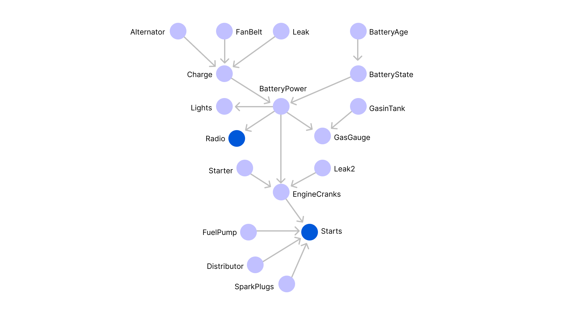
When applied to the accident example, the number of free parameters is equal to 2⁴-1=15. A more complicated example would be trying to model the functioning of a car. If we assume that a car can be broken down to 19 components that can be represented by edges as illustrated in the graph below (which is of course, a gross simplification):

And suppose that we are looking to determine the probability that the car starts, which amounts to computing the marginal probability law of x₁₅ (the blue variable at the bottom).

Once again, for simplicity's sake, we can assume that each variable is binary, indicating whether a given component (e.g., lights) functions or not. In order to derive the marginal probability law of variable x₁₅ , we would need to sum up 2¹⁸ terms (more than 250000 terms!):

Hence, unless we find a different parameterization of the joint probability distribution, the problem is intractable. This is where the information about probabilistic independencies becomes crucial.

To illustrate this, let us reconsider the accident example where the joint probability distribution is given by P(y, x₁, x₂, x₃). Using Bayes rule, we can break down the joint probability distribution into a product of smaller distributions, the key observation being that the total number of free parameters grows additively rather than multiplicatively when we break down the joint distribution, meaning the total number of parameters needed is equal to the sum of the number of parameters needed for each term in the product.

The first distribution is a Bernoulli and can be parametrized by 1 parameter, the second term depends on three binary variables and can thus be parametrized by 2³-1=7 parameters, and the third term depends on two variables and can therefore be parametrized by 2²-1=3 parameters.

Thus, using the dependency structure of the problem, we can reduce the upper bound of the number of values that the joint probability distribution can take, from 15 to 1+7+3=11. This is a very small gain, but when N is large, this simple factorization step can turn the problem from an intractable one to a feasible one, in polynomial time.

In the extreme case where all binary variables are independent, the joint distribution can be rewritten into a product of Bernoulli distributions and the total number of parameters is then N. Hence, the computation complexity of the inference problem would be reduced from exponential to linear in the number of variables.

PGM's in NLP: Hidden Markov Models

In machine learning and statistical inference, we often make the assumptions that the variables, which make up an individual sample, are independent and identically distributed. And while this might be suitable for unstructured tasks like data clustering or survival analysis (where the occurrence of death for an individual patient can be assumed to be independent of his/her cohort), such assumptions are not suitable for sequential data, like the state/evolution of a system over time (e.g., fluctuations of the stock prices) or more importantly: the flow of words in natural language.

A very popular generative model in NLP is the Hidden Markov Model (HMM). Given a set of words (or a vocabulary): V and their corresponding Part of Speech (POS) tags: P, for each time step t ≤ T, we have an observable variable: y_t that is a random variable over V representing the t^th word of a sequence of length T, and that depends on a hidden variable: q_t that represents its POS tag. The HMM representation (MI Jordan, 2003) is illustrated below:

A simple example of an HMM sample would be the sequence: “the cat sleeps”, which would correspond to the variable assignment: (y₁, y₂, y₃) = (“the”, “dog”, “sleeps”) as observables, and (q₁, q₂, q₃) = (Det, Noun, Verb) as hidden variables. The inference problem of an HMM is to approximate the distribution: P (y₁... y_t, q₁... q_t), from a sample of observable variables {(y_1,k ... y_t,k)} where k=1,2.. to N sample size.

A simple version of this model is the trigram HMM, where the state of the current variable q_t is assumed to depend only on the previous two states q_t-1 and q_t-2. Now, let pV be the probability distribution of y_t and p_p be the distribution of q_t. Given an approximation of the trigram probabilities, we can compute the probability of the occurrence of the above sequence following the same recipe as in the previous section:

P (y₁= “the”, y₂= “dog”, y₃= “sleeps”, q₁= Det, q₂= Noun, q₃= Verb)

      = (p_p(q₁= Det). p_p(q₂= Noun | q₁= Det). p_p(q₃= Verb | q₂= Noun, q₁= Det)).

            (p_v(y₁= “the”| q₁= Det). p_v(y₂= “dog”| q₂= Noun). p_v(y₃= “sleeps”| q₃= Verb))

Note that, the connectivity structure of an HMM is, in a sense, trivial. The graph is always a chain; hence the parameter estimation follows the same recipe for any sequence, through the so-called alpha and beta recursions which follow a recursive computation along the chain starting from T. On the other hand, if the graphical model presented loops, standard dynamical programming methods would no longer provide any guarantees, in such cases, the problem would need to be reformulated.

Factor graphs

The popularity of Probabilistic graphical models is at least partly due to the generality of the framework. In fact, to define a PGM over a given set of variables, all we need is a count data of how many times each subset of variables appears together in a sample. And in a number of interesting applications, whether be it in NLP or in computational biology, count data is readily available, which allows us to compute n-grams, or predict linguistic structures, or do topic modelling and much more.

A recurring feature in many complex systems, is that variables can be broken down in several (possibly overlapping) groups, where variables tend to be highly correlated within the same group, but largely independent with the others. In such cases, it can be tricky to work with Markov Networks as they only model dependencies between pairs of variables.

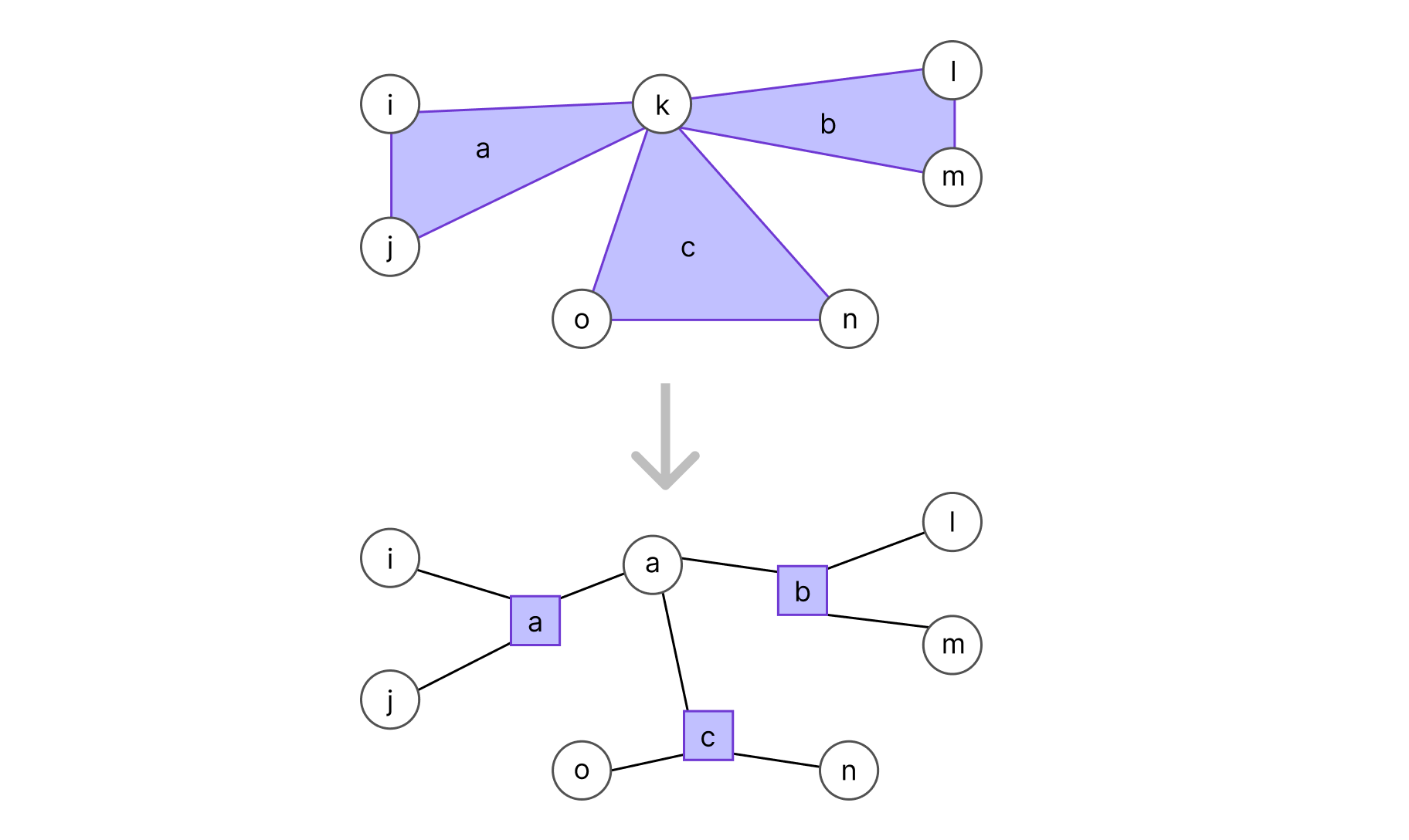
It can then be very useful to use a special class of graphical models called factor graphs. In a factor graph, each group of correlated variables is represented by a function node (a rectangle) that is connected to said variables. These correlated variables form what are called cliques; a clique C is a connected component of a graph: a subset of variables where all variable pairs are connected by an edge:

To transform an undirected graph into a factor graph, for each clique Ca in V we add a function node (represented by a rectangle and linked to every variable in the clique, as shown in the graph below). Conventionally, we should also add a factor for each leaf (omitted to keep the example simple).

Once the dependency structure is assumed, we assign compatibility measures between states or potentials, which are essentially unnormalized probability measures over possible states within cliques. In most applications, the values of potentials for different variable assignments would be extracted from count data.

Consider the example of the factor chain below. If a certain function node a encodes the phenotype of a hidden trait and (x_i , x_j) are the binary variables indicating the presence of some genetic information correlated with the expression of said phenotype and likewise for another phenotype b and its observed variables (x_j , x_k), given some expert information, e.g. the frequency of finding the hidden trait a or b in individuals given the presence of genes (x_i , x_j , x_k), we would have the following potentials:

Note that if the distance between any two variables belonging to different cliques is larger than one (meaning that there is more than one function node along the shortest path) then the two variables are independent, conditioned on their respective clique, which allows us to write P(.) into a product of potentials:

where Z is called the normalization constant and da is the set of variables {x_k} connected to the function node a.

Belief-propagation: A message passing scheme

The next step is to estimate marginals such as: P_i(x_i). However, since the potentials do not necessarily sum to one, the target joint probability distribution P(x₁ ... x_n) is determined only up to the normalization constant Z, such that we would need to normalize it to be able to make inferences.

Assume that all variables share the same support X. To compute the normalization constant, we would need to sum over the entire support: Xⁿ, that is; an exponential number of terms. A key observation is that if the factor graph of our joint probability distribution is a tree, meaning, if the graph does not contain any loops, the following identity holds:

where da is the set of variables that are directly connected to the function node a. This signifies that we could simply compute the normalization constant Z by starting from the leaves and summing the variables at each generation, while taking the product iteratively, all the way up to the root.

The exactitude of this computation is then guaranteed by the following result (Mezard and Montanari, 2009) of which we sketch the proof by the example below.

Proof illustration:

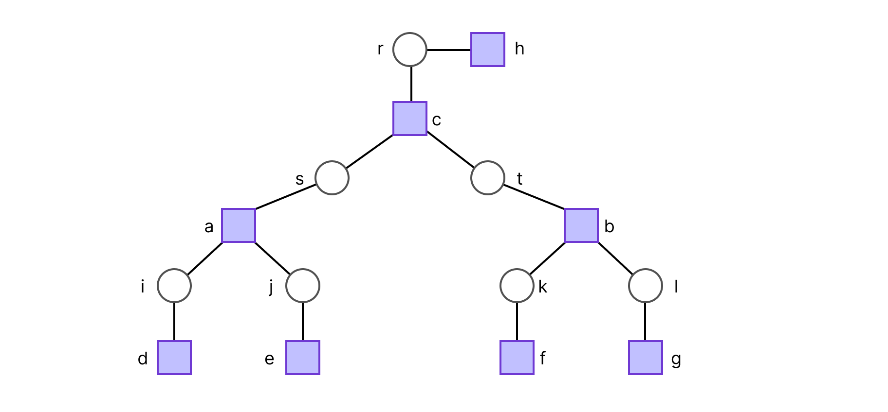
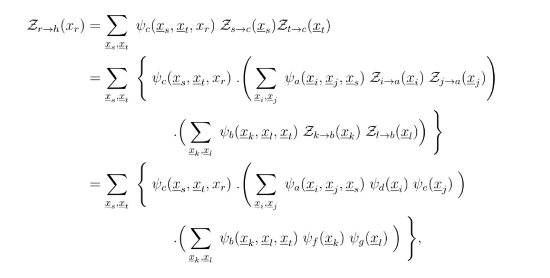
Suppose we chose r to be the root, such that the factor graph is a 2-generation tree. The ideal way to compute Z is to do so in a depth first search fashion. The set of leaf variable nodes is L_v= {r, i, j, k, l}, and following the definition of Z_r→_h(x_r), this results in:

hence

This procedure is very reminiscent of the Viterbi algorithm, and other dynamical programming methods. Once Z is computed, inferences can be made by using the product of the relevant potentials.

References

[2] Mezard M.; Montanari A. 2009. Information, Physics and Computation, Oxford University Press. Sons.